Introduction to Project and Data Management
Computational and data literacy skills for research
15 May 2017, NHM
Session Outline
Research Data Management
Basic Data Hygiene
Metadata
Project Management
File system organisation
File naming
Link to handout: http://bit.ly/NHM_RDM_introduction
The grand vision
Hans Rosling on open data in 2006
How do we get there?
Getting a handle on our research materials
21st Century Research meta-responsibilities
Better digital curation of the workhorses of modern science: code & data
- accessible
- reusable
- searchable
We all need to do our bit

Drivers of better digital management
- Funders: value for money, impact, reputation
- Publishers: many now require code and data.
- Specialist journals for software (e.g Journal of Open Source Software and data (e.g. Scientific Data) have emerged.
- Your wider scientific community
- PIs, Supervisors and immediate research group
Yourselves!
be your own best friend:
aim to create secure materials that are easy to use and REUSE
Resources
Nine simple ways to make it easier to (re)use your data
We describe nine simple ways to make it easy to reuse the data that you share and also make it easier to work with it yourself. Our recommendations focus on making your data understandable, easy to analyze, and readily available to the wider community of scientists.

BES guide to data management
This guide for early career researchers explains what data and data management are, and provides advice and examples of best practices in data management, including case studies from researchers currently working in ecology and evolution.


Data carpentry
- Domain specific lessons available free online
- Ecology materials
- Genomics materials
- Geospatial data materials
- Biology semester long materials
- Look out for training sessions
Seek help from support teams
Most university libraries have assistants dedicated to Research Data Management:
@tomjwebb @ScientificData Talk to their librarian for data management strategies #datainfolit
— Yasmeen Shorish (@yasmeen_azadi) January 16, 2015
Basic Data Hygiene
Plan your Research Data Management
- Start early. Make an RDM plan before collecting data.
- Anticipate data products as part of your thesis outputs
- Think about what technologies to use
Take initiative & responsibility. Think long term.
Act as though every short term study will become a long term one @tomjwebb. Needs to be reproducible in 3, 20, 100 yrs
— oceans initiative (@oceansresearch) January 16, 2015
Data entering
extreme but in many ways defendable
@tomjwebb stay away from excel at all costs?
— Timothée Poisot (@tpoi) January 16, 2015
excel: read only
@tomjwebb @tpoi excel is fine for data entry. Just save in plain text format like csv. Some additional tips: pic.twitter.com/8fUv9PyVjC
— Jaime Ashander (@jaimedash) January 16, 2015
@jaimedash just don’t let excel anywhere near dates or times. @tomjwebb @tpoi @larysar
— Dave Harris (@davidjayharris) January 16, 2015
Databases: more robust
- good qc and advisable for multiple contributors
@tomjwebb databases? @swcarpentry has a good course on SQLite
— Timothée Poisot (@tpoi) January 16, 2015
@tomjwebb @tpoi if the data are moderately complex, or involve multiple people, best to set up a database with well designed entry form 1/2
— Luca Borger (@lucaborger) January 16, 2015
Databases: benefits
@tomjwebb Entering via a database management system (e.g., Access, Filemaker) can make entry easier & help prevent data entry errors @tpoi
— Ethan White (@ethanwhite) January 16, 2015
@tomjwebb it also prevents a lot of different bad practices. It is possible to do some of this in Excel. @tpoi
— Ethan White (@ethanwhite) January 16, 2015
@ethanwhite +1 Enforcing data types, options from selection etc, just some useful things a DB gives you, if you turn them on @tomjwebb @tpoi
— Gavin Simpson (@ucfagls) January 16, 2015
Data formats
.csv: comma separated values..tsv: tab separated values..txt: no formatting specified.
@tomjwebb It has to be interoperability/openness - can I read your data with whatever I use, without having to convert it?
— Paul Swaddle (@paul_swaddle) January 16, 2015
more unusual formats will need instructions on use.
Ensure data is machine readable
bad

bad

good

ok

- could help data entry
.csvor.tsvcopy would need to be saved.
Use good null values
Missing values are a fact of life
- Usually, best solution is to leave blank
NAorNULLare also good options- NEVER use
0. Avoid numbers like-999 - Don’t make up your own code for missing values
read.csv() utilities
na.string: character vector of values to be coded missing and replaced withNAto argument egstrip.white: Logical. ifTRUEstrips leading and trailing white space from unquoted character fieldsblank.lines.skip: Logical: ifTRUEblank lines in the input are ignored.fileEncoding: if you’re getting funny characters, you probably need to specify the correct encoding.
read.csv(file, na.strings = c("NA", "-999"), strip.white = TRUE,
         blank.lines.skip = TRUE, fileEncoding = "mac")
readr::read_csv() utilities
na: character vector of values to be coded missing and replaced withNAto argument egtrim_ws: Logical. ifTRUEstrips leading and trailing white space from unquoted character fieldscol_types: Allows for column data type specification. (see more)locale: controls things like the default time zone, encoding, decimal mark, big mark, and day/month namesskip: Number of lines to skip before reading data.n_max: Maximum number of records to read.
read_csv(file, col_names = TRUE, col_types = NULL, locale = default_locale(),
         na = c("", "NA", "-999"), trim_ws = TRUE, skip = 0, n_max = Inf)
Basic quality control
Have a look at your data with Viewer(df)
- Check empty cells
- Check the range of values (and value types) in each column matches expectation. Use
summary(df) - Check units of measurement
- Check your software interprets your data correctly eg.
for a data framedf;head(df)(see top few rows) andstr(df)(see object structure) are useful.
- consider writing some simple QA tests (eg. checks against number of dimensions, sum of numeric columns etc)
Raw data are sacrosanct
@tomjwebb don't, not even with a barge pole, not for one second, touch or otherwise edit the raw data files. Do any manipulations in script
— Gavin Simpson (@ucfagls) January 16, 2015
@tomjwebb @srsupp Keep one or a few good master data files (per data collection of interest), and code your formatting with good annotation.
— Desiree Narango (@DLNarango) January 16, 2015
Know your masters
- identify the
mastercopy of files - keep it safe and and accessible
- consider version control
- consider centralising

Avoid catastrophe
Backup: on disk
- consider using backup software like Time Machine (mac) or File History (Windows 10)
Backup: in the cloud
- dropbox, googledrive etc.
- if installed on your system, can programmatically access them through
R - some version control
@tomjwebb Back it up
— Ben Bond-Lamberty (@BenBondLamberty) January 16, 2015
Backup: the Open Science Framework osf.io
- version controlled
- easily shareable
- works with other apps (eg googledrive, github)
- work on an interface with R (OSFr) is in progress. See more here
Backup: Github
most solid version control.
keep everything in one project folder.
Can be problematic with really large files.
Metadata
Documenting your data
You got data. Is it enough?
@tomjwebb I see tons of spreadsheets that i don't understand anything (or the stduent), making it really hard to share.
— Erika Berenguer (@Erika_Berenguer) January 16, 2015
@tomjwebb @ScientificData “Document. Everything.” Data without documentation has no value.
— Sven Kochmann (@indianalytics) January 16, 2015
@tomjwebb Annotate, annotate, annotate!
— CanJFishAquaticSci (@cjfas) January 16, 2015
Document all the metadata (including protocols).@tomjwebb
— Ward Appeltans (@WrdAppltns) January 16, 2015
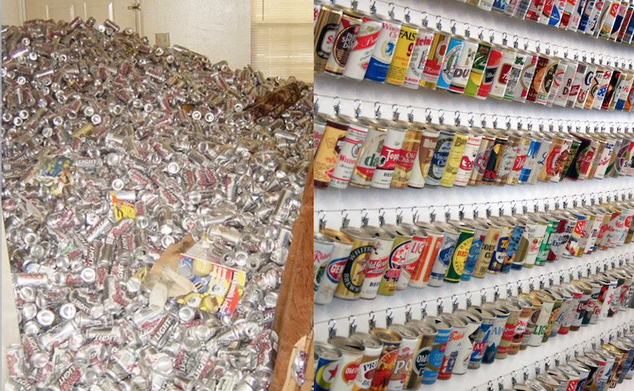
You download a zip file of #OpenData. Apart from your data file(s), what else should it contain?
— Leigh Dodds (@ldodds) February 6, 2017
#otherpeoplesdata dream match!
Thought experiment: Imagine a dream open data set
It’s out there somewhere:
How would you locate it?
- what details would you need to know to determine relevance?
- what information would you need to know to use it?
metadata = data about data
Information that describes, explains, locates, or in some way makes it easier to find, access, and use a resource (in this case, data).

Backbone of digital curation
Without it a digital resource may be irretrievable, unidentifiable or unusable
Descriptive
- enables identification, location and retrieval of data, often includes use of controlled vocabularies for classification and indexing.
Technical
- describes the technical processes used to produce, or required to use a digital data object.
Administrative
- used to manage administrative aspects of the digital object e.g. intellectual property rights and acquisition.
This usually takes the form of a structured set of elements.
Elements of metadata
Structured data files:
- readable by machines and humans, accessible through the web
Controlled vocabularies eg. NERC Vocabulary server
- allows for connectivity of data
KEY TO SEARCH FUNCTION
- By structuring & adhering to controlled vocabularies, data can be combined, accessed and searched!
- Different communities develop different standards which define both the structure and content of metadata
Organising data and metadata
Start at the very least by creating a metadata tab within your raw data spreadsheets
Ideally set up a system of normalised tables (see section 3 in this post) and
READMEdocuments to manage and document metadata.Ensure everything someone might need to understand your data is documented
Different types data require different metadata
When you’re ready to publish, structure metadata into an
XMLfile, a searchable, shareable file.
Make your data alignable and generalisable
What information would other users need to combine your data with theirs?
- time
temporal (time of day, day, month, year, season) - space
geography (lat, lon, postcode) - taxonomy
species name; authority / source - provide information on extent and resolution
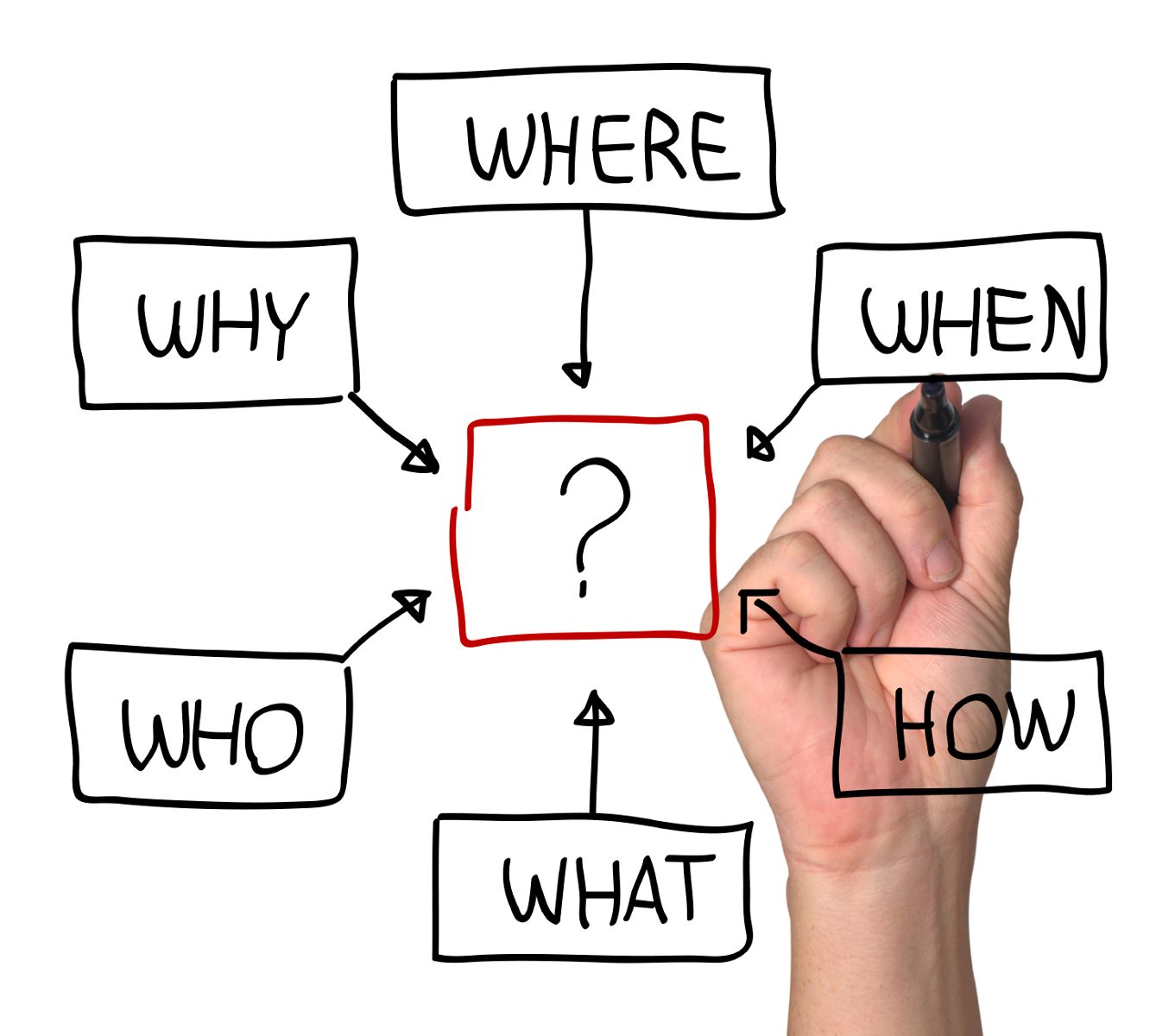
@tomjwebb record every detail about how/where/why it is collected
— Sal Keith (@Sal_Keith) January 16, 2015
Example metadata structure
Bird Trait Networks dataset
I’m using data from a project in which we compiled large dataset on bird reproductive, morphological, physiological, life history and ecological traits across as many bird species as possible to perform a network analysis on associations between trait pairs.
I’ll use a simplified subset of the data to show a simple metadata (attribute) structure that can easily form the basis of a more formal EML (ecological XML) using function in the package EML
Data
| species | max.altitude | dev.mode | courtship.feed.m | song.dur | breed.system |
|---|---|---|---|---|---|
| Acridotheres_tristis | NA | 2 | 0 | NA | 1 |
| Aix_galericulata | NA | 1 | NA | NA | 2 |
| Anas_americana | NA | 1 | NA | NA | 2 |
| Anas_clypeata | NA | 1 | NA | NA | 2 |
| Anthracothorax_nigricollis | NA | 2 | NA | NA | 2 |
| Anthus_hodgsoni | NA | 2 | NA | NA | 1 |
| Aphelocoma_coerulescens | NA | 2 | NA | NA | 4 |
| Aphelocoma_ultramarina | NA | 2 | NA | NA | NA |
| Ardea_cinerea | NA | 2 | NA | NA | 1 |
Like many real data sets, column headings are convenient for data entry and manipulation, but not particularly descriptive to a user not already familiar with the data.
More importantly, they don’t let us know what units they are measured in (or in the case of categorical / factor data, what the factor abbreviations refer to). So let us take a moment to be more explicit:
Make an attribute table
I use functions in eml_utils.R to:
- create an
attr_tblin which to complete all info required - to extract elements from
attr_tblto supply to EML generating functions.
library(RCurl)
eval(parse(text = getURL(
    "https://raw.githubusercontent.com/annakrystalli/ACCE_RDM/master/R/eml_utils.R",
    ssl.verifypeer = FALSE)))
Create attr_tbl shell
load data
dt <- read.csv("data/bird_trait_db-v0.1.csv")create
attr_tblshell from your data (dt)- use function
get_attr_shellfromeml_utils.R.
- use function
attr_shell <- get_attr_shell(dt)attr_tbl shell structure
str(attr_shell)## 'data.frame': 6 obs. of 11 variables:
## $ attributeName : chr "species" "max.altitude" "dev.mode" "courtship.feed.m" ...
## $ attributeDefinition: logi NA NA NA NA NA NA
## $ columnClasses : chr "character" "numeric" "numeric" "numeric" ...
## $ numberType : logi NA NA NA NA NA NA
## $ unit : logi NA NA NA NA NA NA
## $ minimum : logi NA NA NA NA NA NA
## $ maximum : logi NA NA NA NA NA NA
## $ formatString : logi NA NA NA NA NA NA
## $ definition : logi NA NA NA NA NA NA
## $ code : logi NA NA NA NA NA NA
## $ levels : logi NA NA NA NA NA NA
attributes df columns
I use recognized column headers shown here to make it easier to create an EML object down the line. I focus on the core columns required but you can add additional ones for your own purposes.
Attributes associated with all variables:
- attributeName (required, free text field)
- attributeDefinition (required, free text field)
- columnClasses (required,
"numeric","character","factor","ordered", or"Date", case sensitive)
columnClasses dependant attributes
- For
numeric(ratio or interval) data:- unit (required, see eml-unitTypeDefinitions and working with units)
- For
character(textDomain) data:- definition (required)
- For
dateTimedata:- formatString (required) e.g for date
11-03-2001formatString would be"DD-MM-YYYY"
- formatString (required) e.g for date
- I use the columns
codeandlevelsto store information on factors. Use";"to separate code and level descriptions. These can be extracted byeml_utils.Rfunctionget_attr_factors()later on.
Complete attr_tbl
save shell
- write
attr_shellto.csv
write.csv(attr_shell, file = "data/attr_shell.csv")complete attr_tbl
- complete in your prefered spreadsheet editing software and save to attr_tbl.csv
- read in completed attr_tbl.csv
attr_tbl <- read.csv(file = "data/attr_tbl.csv")
Completed attribute table attr_tbl
| attributeName | attributeDefinition | columnClasses | numberType | unit | minimum | maximum | formatString | definition | code | levels |
|---|---|---|---|---|---|---|---|---|---|---|
| species | species | character | NA | NA | NA | NA | NA | species | NA | NA |
| max.altitude | Maximum altitudinal distribution | numeric | integer | meter | NA | NA | NA | NA | NA | NA |
| dev.mode | Developmental mode | ordered | NA | NA | NA | NA | NA | NA | 1;2;3 | Altricial;Semiprecocial;Precocial |
| courtship.feed.m | Courtship feeding (by the male) | factor | NA | NA | NA | NA | NA | Courtship feeding (by the male) | 0;1 | FALSE;TRUE |
| song.dur | Song duration | numeric | real | second | 0 | NA | NA | NA | NA | NA |
| breed.system | Which adult(s) provides the majority of care: | factor | NA | NA | NA | NA | NA | Breeding system | 1;2;3;4;5 | Pair;Female;Male;Cooperative;Occassional |
Project Organisation
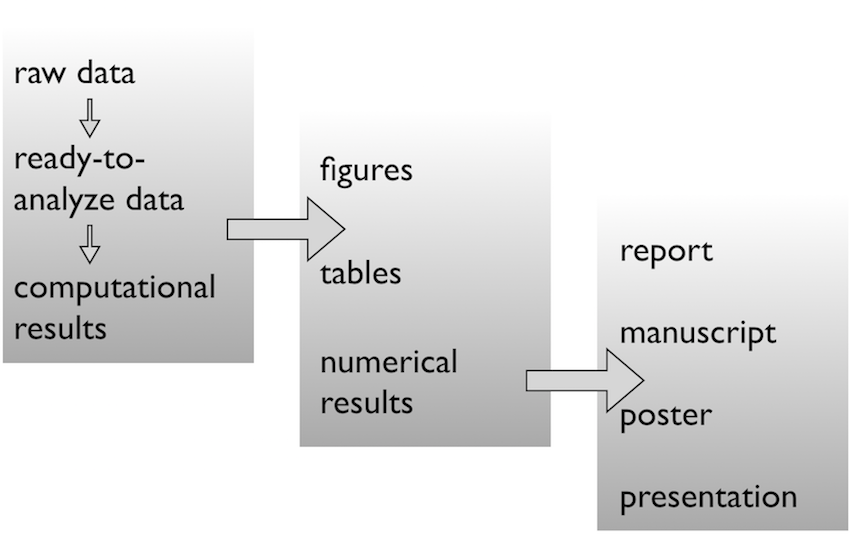
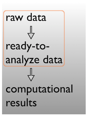
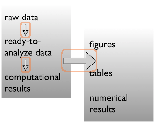
From raw to analytical data
the reproducible pipeline
Do not manually edit raw data
Keep a clean pipeline of data processing from raw to analytical.

- Ideally, incorporate checks to ensure correct processing of data through to analytical.
Automated == reproducible
HOW?
Let’s face it…
There are going to be files
LOTS of files
The files will change over time
The files will have relationships to each other
It’ll probably get complicated
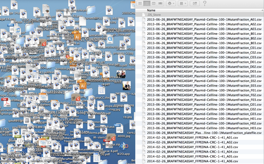
Strategy against chaos
File organization and naming is a mighty weapon against chaos
- Make a file’s name and location VERY INFORMATIVE about:
- what it is,
- why it exists,
- how it relates to other things
The more things are self-explanatory, the better
READMEs are great, but don’t document something if you could just make that thing self-documenting by definition
File system organisation
A place for everything, everything in its place.
Benjamin Franklin
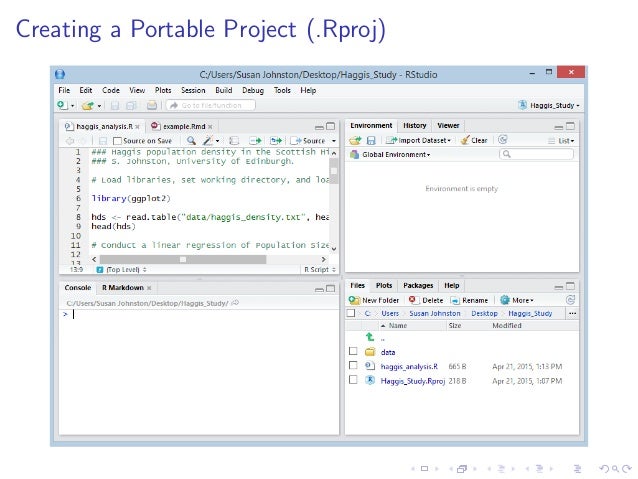
Use R projects
Data analysis workflow
Use sensible / standardised file system structure
 source: https://nicercode.github.io/blog/2013-04-05-projects/
Raw data \(\rightarrow\) data
Pick a strategy, any strategy, just pick one!
data/
data-raw
data-clean

data/
  - raw/
  - clean/
Data \(\rightarrow\) results
Pick a strategy, any strategy, just pick one!
R

code

scripts

analysis

bin
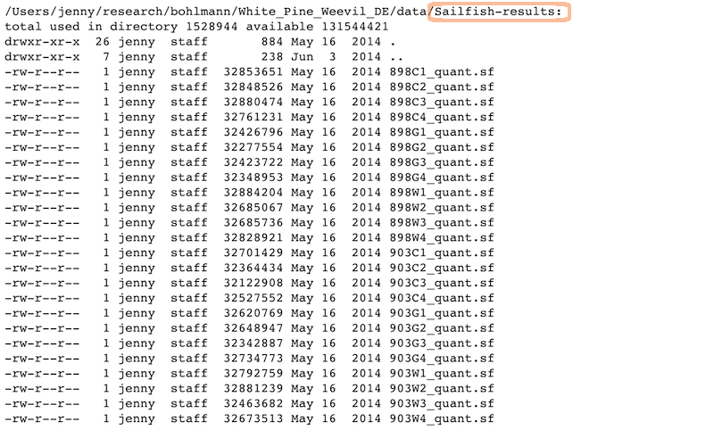
A real (and imperfect!) example
  /Users/jenny/research/bohlmann/White_Pine_Weevil_DE:
  total used in directory 246648 available 131544558
  drwxr-xr-x  14 jenny  staff        476 Jun 23  2014 .
  drwxr-xr-x   4 jenny  staff        136 Jun 23  2014 ..
  -rw-r--r--@  1 jenny  staff      15364 Apr 23 10:19 .DS_Store
  -rw-r--r--   1 jenny  staff  126231190 Jun 23  2014 .RData
  -rw-r--r--   1 jenny  staff      19148 Jun 23  2014 .Rhistory
  drwxr-xr-x   3 jenny  staff        102 May 16  2014 .Rproj.user
  drwxr-xr-x  17 jenny  staff        578 Apr 29 10:20 .git
  -rw-r--r--   1 jenny  staff         50 May 30  2014 .gitignore
  -rw-r--r--   1 jenny  staff       1003 Jun 23  2014 README.md
  -rw-r--r--   1 jenny  staff        205 Jun  3  2014 White_Pine_Weevil_DE.Rproj
  drwxr-xr-x  20 jenny  staff        680 Apr 14 15:44 analysis/
  drwxr-xr-x   7 jenny  staff        238 Jun  3  2014 data/
  drwxr-xr-x  22 jenny  staff        748 Jun 23  2014 model-exposition/
  drwxr-xr-x   4 jenny  staff        136 Jun  3  2014 results/
Data
Ready to analyze data:
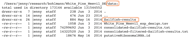
Raw data:
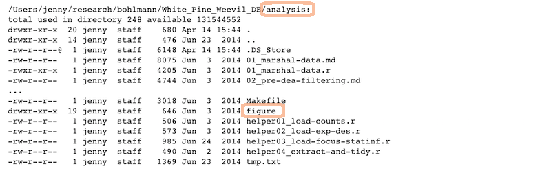
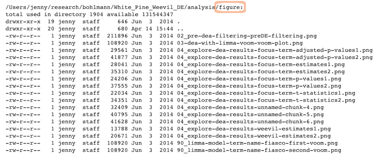
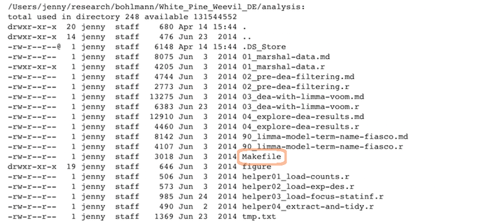
Analysis and figures
R scripts + the Markdown files:
sample_ready_to_analyze_data
The figures created in those R scripts and linked in those Markdown files:
sample_raw_data
Scripts
Linear progression of R scripts, and Makefile to run the entire analysis:
sample_scripts
Results
Tab-delimited files with one row per gene of parameter estimates, test statistics, etc.:
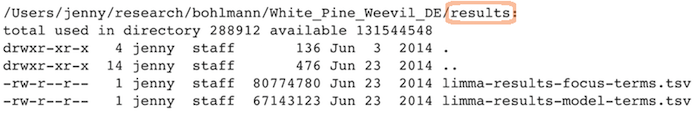
sample_results
Expository files
Files to help collaborators understand the model we fit: some markdown docs, a Keynote presentation, Keynote slides exported as PNGs for viewability on GitHub:
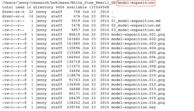
sample_expository
Caveats / problems with this example
This project is nowhere near done, i.e. no manuscript or publication-ready figs
File naming has inconsistencies due to three different people being involved
Code and reports/figures all sit together because it’s just much easier that way w/
knitr&rmarkdown
Wins of this example
Someone can walk away from the project and come back to it a year later and resume work fairly quickly
Collaborators (the two other people, the post-doc whose project it is + the bioinformatician for that lab) were able to figure out what I did and decide which files they needed to look at, etc.
More project management tips
Evolution of your file system
Be consistent – when developing a naming scheme for folders it is important that once you have decided on a method, you stick to it. If you can, try to agree on a naming scheme from the outset of your research project
Structure folders hierarchically: - start with a limited number of folders for the broader topics - create more specific folders within these
Separate ongoing and completed work: as you start to create lots of folders and files, it is a good idea to think about separating older documents from those you are currently working on
The from_joe directory
Let’s say your collaborator and data producer is Joe.
He will send you data with weird space-containing file names, data in Microsoft Excel workbooks, etc.
It is futile to fight this, just quarantine all the crazy in a
from_joedirectory.Rename things and/or export to plain text and put those files in your data directory.
Record whatever you do you do to those inputs in a README or in comments in your R code

Give yourself less rope
It’s a good idea to revoke your own write permission to the raw data file.
Then you can’t accidentally edit it.
It also makes it harder to do manual edits in a moment of weakness, when you know you should just add a line to your data cleaning script.
Prose
Sometimes you need a place to park key emails, internal documentation and explanations, random Word and PowerPoint docs people send, etc.
This is kind of like
from_joe, where I don’t force myself to keep same standards with respect to file names and open formats.
Recap
File organization should reflect inputs vs outputs and the flow of information
/Users/jenny/research/bohlmann/White_Pine_Weevil_DE:
drwxr-xr-x  20 jenny  staff        680 Apr 14 15:44 analysis
drwxr-xr-x   7 jenny  staff        238 Jun  3  2014 data
drwxr-xr-x  22 jenny  staff        748 Jun 23  2014 model-exposition
drwxr-xr-x   4 jenny  staff        136 Jun  3  2014 results
Prepare data \(\rightarrow\) Do stats \(\rightarrow\) Make tables & figs
The R scripts:
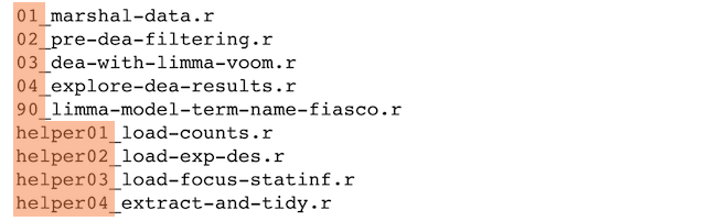
01_marshal-data.r
02_pre-dea-filtering.r
03_dea-with-limma-voom.r
04_explore-dea-results.r
90_limma-model-term-name-fiasco.r
The figures left behind:
02_pre-dea-filtering-preDE-filtering.png
03-dea-with-limma-voom-voom-plot.png
04_explore-dea-results-focus-term-adjusted-p-values1.png
04_explore-dea-results-focus-term-adjusted-p-values2.png
...
90_limma-model-term-name-fiasco-first-voom.png
90_limma-model-term-name-fiasco-second-voom.png
File naming
Names matter

What works, what doesn’t?
NO
myabstract.docx
Joe’s Filenames Use Spaces and Punctuation.xlsx
figure 1.png
fig 2.png
JW7d^(2sl@deletethisandyourcareerisoverWx2*.txt
YES
2014-06-08_abstract-for-sla.docx
joes-filenames-are-getting-better.xlsx
fig01_scatterplot-talk-length-vs-interest.png
fig02_histogram-talk-attendance.png
1986-01-28_raw-data-from-challenger-o-rings.txt
Three principles for (file) names
1. Machine readable
2. Human readable
3. Plays well with default ordering
Awesome file names :)
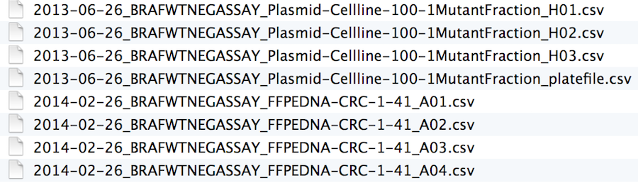
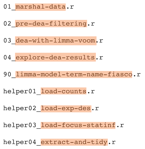
Machine readable
- Regular expression and globbing friendly
- Avoid spaces, punctuation, accented characters, case sensitivity
- Easy to compute on
- Deliberate use of delimiters
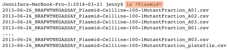
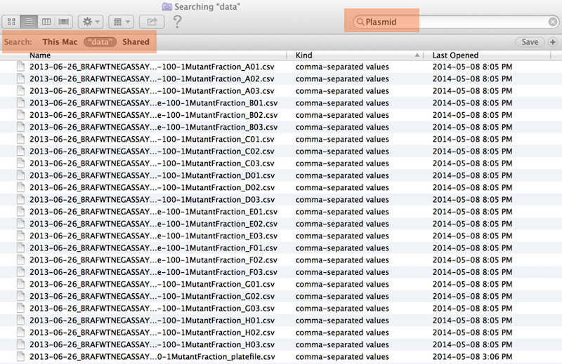
Same using Mac OS Finder search facilities
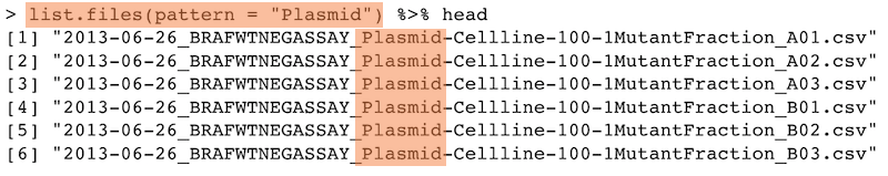
Same using regex in R
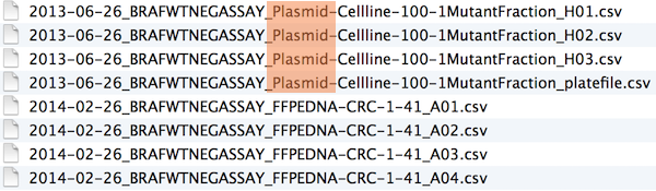
Punctuation
Deliberate use of "-" and "_" allows recovery of meta-data from the filenames:
"_"underscore used to delimit units of meta-data I want later"-"hyphen used to delimit words so my eyes don’t bleed
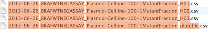
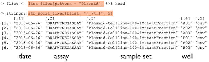
This happens to be R but also possible in the shell, Python, etc.
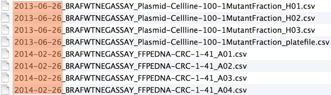
Include important metadata
e.g. I’m saving a number of files of extracted environmental data at different resolutions (res) and for a number of months (month).
write.csv(df, paste("variable_", res, month, sep ="_"))

df <- read.csv(paste("variable_", res, month, sep ="_"))
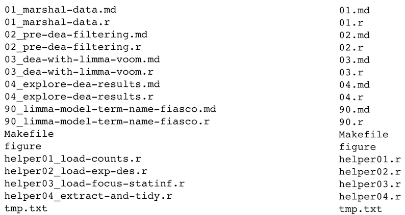
Recap: machine readable
- Easy to search for files later
- Easy to narrow file lists based on names
- Easy to extract info from file names, e.g. by splitting
- New to regular expressions and globbing? be kind to yourself and avoid
- Spaces in file names
- Punctuation
- Accented characters
Human readable
Example
Which set of file(name)s do you want at 3 a.m. before a deadline?
Embrace the slug

Recap: Human readable
\(\rightarrow\) Easy to figure out what the heck something is, based on its name
Plays well with default ordering
Plays well with default ordering
- Put something numeric first
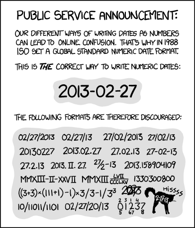
- Use the ISO 8601 standard for dates
- Left pad other numbers with zeros
Examples
Chronological order:
Logical order: Put something numeric first
Dates
Use the ISO 8601 standard for dates: YYYY-MM-DD
Left pad other numbers with zeros
If you don’t left pad, you get this:
10_final-figs-for-publication.R
1_data-cleaning.R
2_fit-model.R
which is just sad :(
Recap: Plays well with default ordering
Put something numeric first
Use the ISO 8601 standard for dates
Left pad other numbers with zeros
Recap: Three principles for (file) names
Machine readable
Human readable
Plays well with default ordering
Go forth and use awesome file names :)
chronological_order
logical_order
Let’s set up our project!
Activity : Create an RStudio project
- Create an project in which we will work this week
- Create a data folder
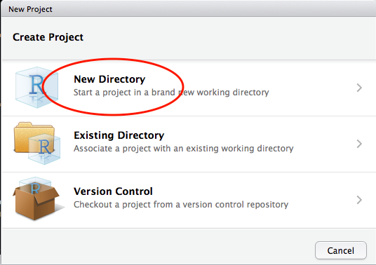
New Directory
File -> New Project -> New Directory
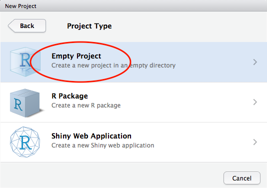
Empty Project
In the Project Type screen, click on Empty Project.
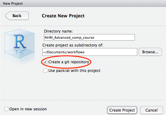
Name project directory
In the Create New Project screen, give your project a name and ensure that create a git repository is checked. Click on Create Project.
New project directory created
RStudio will create a new folder containing an empty project and set R’s working directory to within it.
Two files are created in the otherwise empty project:-
- .gitignore - Specifies files that should be ignored by the version control system.
- NHM_Advanced_comp_course.Rproj - Configuration information for the RStudio project
There is no need to worry about the contents of either of these for now.
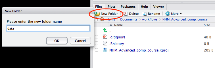
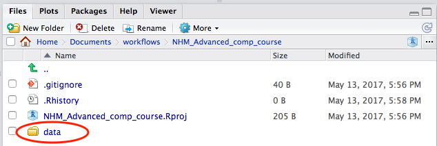
Create a data folder
Success!
Acknowledgements
Materials remixed from:
ACCE Research Data Management workshop materials
Data carpentry File Organization workshop materials